CS342 Machine Learning
Lecture 1 – January 8th, 2018
Ask questions on the Machine Learning forum, if you can, instead of emailing Theo directly.
Assessment
-
Final Exam (60%), based on lecture material & PPs & worksheets
-
Coursework (40%):
- First assignment (15%).
- Second assignment (25%), on a real-world ML competition platform.
Syllabus
- A First Course in Machine Learning, 2nd Edition, S. Rogers & M. Girolami
- Machine Learning, T. Mitchell
How does one learn?
-
Supervised learning
- Direct feedback: car is blue, car is red, car is red, etc…
- Indirect reward feedback: better, worse, hot cold, etc… (e.g. dopamine)
-
Unsupervised learning
- Creating clusters or groups, finding patterns in data with no direct goal for what constitutes the right pattern to spot.
The common goal of ML systems
-
They learn from data (“experience” ).
-
A computer program is said to learn from experience E (data) with respect to some class of tasks T and performance measure P, if its performance at tasks in T, as measured by P, improves with experience E.
Main subfields of ML
-
Supervised
- Regression
- Classification
- Ranking
- Structured Prediction
-
Unsupervised
- Clustering
- Dimensionality Reduction (100x100 image is a vector in a 10000 dimensional space, which needs to be reduced to work with)
- Manifold Learning
-
Reinforcement
- Markov Decision Process (e.g. Robotics)
- Multi-Agent Systems
- TD/Q-Learning (State-Action-Reward)
Regression
Lecture 2 – January 11th, 2018
Conventionally, in Computer Science, you have your program and input as input to the computer, and you have your output as output. With supervised learning, you have your input and output as input, and you have your program as output.
Hypotheses: the relationship between X and t is linear.
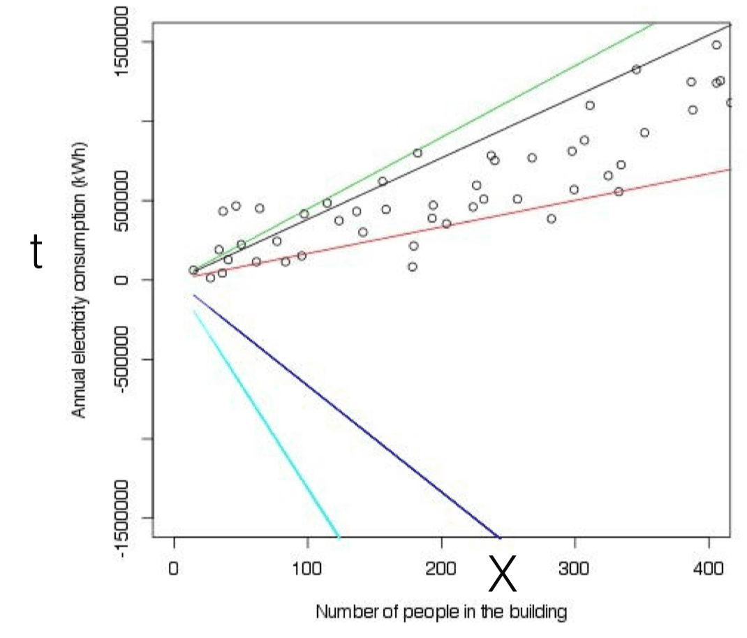
What are the best parameters? Somewhere between the black and the red line we must have a measure of goodness of fit that we try and maximize.
To generalize:
Data: input / outputs .
Parameters: .
Hypothesis space: .
“Goodness” metric: e.g. the distance between and .
Note: you don’t have to run your learning algorithms on the raw input. By intelligently preprocessing raw data so that you end up with a smaller feature set, you can end up with a more effective result. The concept of creating features from inputs is called feature engineering.
Goodness metrics
Squared loss:
Absolute difference:
So, what we’re looking for:
Approach:
- Replace the expression with a specific loss function.
- Equate first derivative of loss to zero to get (find potential minima).
- Examine second derivative of loss at to determine if unique minima.
Lecture 3 – January 12th, 2018
Missed.
Lecture 4 – January 15th, 2018
Missed.
Lecture 5 – January 18th, 2018
Euclidean vs. Manhattan distance.
Manhattan: you can’t walk diagonally (as the crow flies).
With Manhattan distance, when deciding on boundaries based on distances to points, you may end up with boundaries which are equidistant to two points.
Distance-weighted k-NN
- Weigh the vote of each neighbour by its distance to the observation. The further away it is, the less it gets counted for.
- Can help break ties when k is even.
- Can help deal with noisy data and outliers
Lecture 6 – January 19th, 2018
Missed lecture.
Lecture 7 – January 22nd, 2018
Classification: Binary and Multi-class (Multinomial)
For binary classifying, you have True Positives, True Negatives for correct classifying, and False Positives, and False Negatives for incorrect classification.
You might want to care more about false negatives than false positives. This must be stated in how you measure loss (weighing false negatives more heavily).
The ROC Curve: Receiver Operating Characteristic curve
Ridge regression
To reduce the size of the parameter space you can penalise large parameters by including them in your loss function. By picking different norms you’ll end up with different results. Ridge regression uses the L2 ball, for the Lasso you use the L1 ball, which works well for sparse high dimensional data.
Lecture 8 – January 25th, 2018
No notes.
Lecture 9 – January 26th, 2018
Missed lecture.
Lecture 10 – January 29th, 2018
Improved k-NN
A weighted distance function:
Bias-Variance decomposition
Trivial…
Lecture 11 – February 1st, 2018
By only getting and throwing away all the other potential solutions, you don’t know about the stability of the solutions.
Bayesian Inference
Idea: treat as a random variable. E.g. .
Lecture 12 – February 2nd, 2018
Missed lecture.